Regressionsdiagnostik in R

Einen ausgezeichneten Überblick über die Regressionsdiagnostik gibt John Fox in seinem treffend benannten Überblick über die Regressionsdiagnostik. Dr. Das Auto-Paket von Fox bietet fortschrittliche Hilfsmittel für die Regressionsmodellierung.

# Assume that we are fitting a multiple linear regression
#
on the MTCARS data
library(car)
fit <- lm(mpg~disp+hp+wt+drat, data=mtcars)

Dieses Beispiel dient nur zur Veranschaulichung. Wir werden die Tatsache ignorieren, dass dies möglicherweise keine gute Methode zur Modellierung dieses speziellen Datensatzes ist!

Ausreißer

# Assessing Outliers
outlierTest(fit) # Bonferonni p-value for most extreme obs
qqPlot(fit, main="QQ Plot") #qq plot for studentized resid

leveragePlots(fit) # leverage plots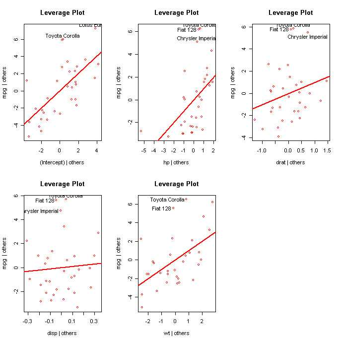

Einflussreiche Beobachtungen

# Influential Observations
# added variable plots
av.Plots(fit)
# Cook's D plot
# identify D values > 4/(n-k-1)
cutoff <- 4/((nrow(mtcars)-length(fit$coefficients)-2))
plot(fit, which=4, cook.levels=cutoff)
# Influence Plot

influencePlot(fit, id.method="identify", main="Influence Plot", sub="Circle size is proportial to Cook's Distance" )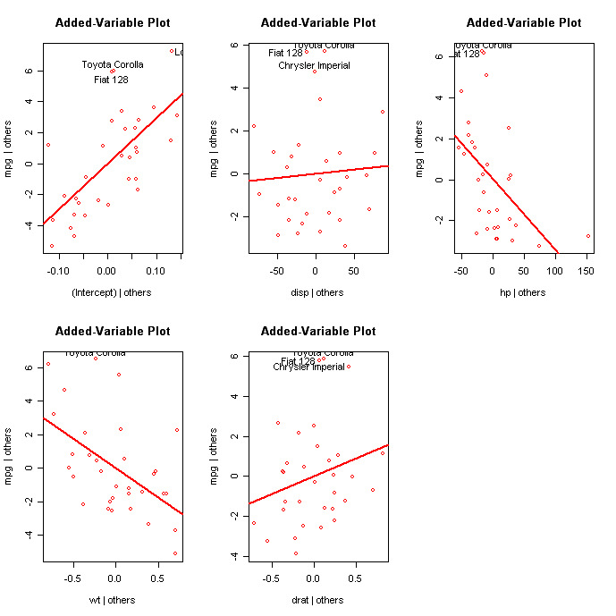

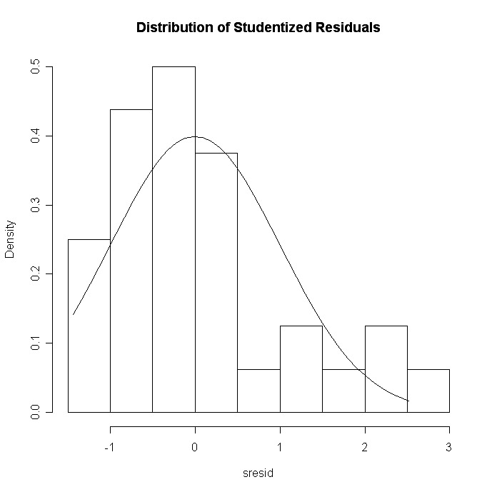
Nicht-Normalität

# Normality of Residuals
# qq plot for studentized resid
qqPlot(fit, main="QQ Plot")
# distribution of studentized residuals
library(MASS)
sresid <- studres(fit)
hist(sresid, freq=FALSE,
   main="Distribution of Studentized Residuals")
xfit<-seq(min(sresid),max(sresid),length=40)
yfit<-dnorm(xfit)

lines(xfit, yfit)

Nicht konstante Fehlervarianz

# Evaluate homoscedasticity
# non-constant error variance test
ncvTest(fit)
# plot
studentized residuals vs. fitted values
spreadLevelPlot(fit)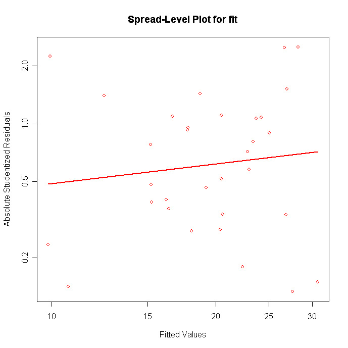

Multikollinearität

# Evaluate Collinearity
vif(fit) # variance inflation factors
sqrt(vif(fit)) > 2 # problem?

Nichtlinearität

# Evaluate Nonlinearity
# component + residual plot
crPlots(fit)
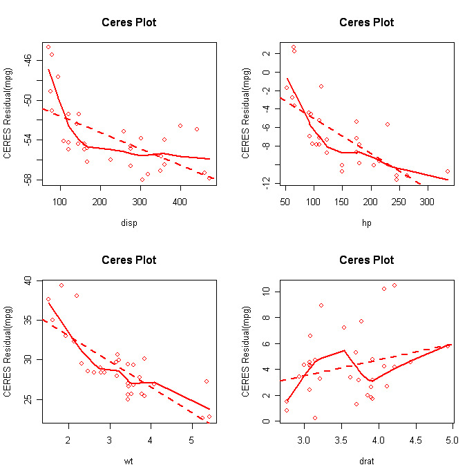
# Ceres plots
ceresPlots(fit)

Nicht-Unabhängigkeit von Fehlern

# Test for Autocorrelated Errors
durbinWatsonTest(fit)

Zusätzliche diagnostische Hilfe

Die Funktion gvlma( ) im gvlma-Paket führt eine globale Validierung der Annahmen des linearen Modells sowie separate Bewertungen der Schiefe, Kurtosis und Heteroskedastizität durch.

# Global test of model assumptions
library(gvlma)
gvmodel <- gvlma(fit)

summary(gvmodel)

Weiter gehen

Wenn du tiefer in die Regressionsdiagnostik einsteigen möchtest, helfen dir zwei Bücher von John Fox: Applied regression analysis and generalized linear models (2nd ed) und An R and S-Plus companion to applied regression.