Box-Cox Transformation: Stabilize Variance Without Guessing

You're building a linear regression model on housing prices. The residual plot looks like a megaphone (narrow on the left, spreading wide on the right). The model technically runs. The results are just not reliable. That pattern is heteroscedasticity, and it's one of those violations that quietly invalidates your inferences without throwing an obvious error.

One option is to transform the response variable. And instead of guessing whether to try a log, a square root, or a reciprocal, you can let the data suggest the right one. That's the idea behind the Box-Cox transformation, and it's what we'll cover here: the formula, how to choose lambda, and how to implement it in Python and R.

What Is the Box-Cox Transformation?

The Box-Cox transformation is a family of power transformations for strictly positive data. Rather than picking a specific transformation yourself, it gives you a way to search across a whole range of them, each indexed by a parameter called lambda (λ).

When lambda equals 0, you get a log transformation. When it equals 0.5, you get something close to a square root. When it equals -1, you're near a reciprocal. All of these are special cases of the same formula, which means you don't have to choose between them ahead of time. You estimate which one fits best from the data.

One thing worth being clear about from the start: Box-Cox doesn't just "make data normal." Depending on your modeling problem, it can help stabilize variance, improve linearity between predictors and the response, or better satisfy your model's assumptions. It also requires strictly positive input values. Zeros and negatives are out. More on that in the limitations section.

How the Box-Cox Transformation Works

Before the formula, it's worth building some intuition. Say you have a variable like weekly sales revenue and it's right-skewed: a long tail to the right, variance that grows with the mean. The question is what power of that variable behaves more like a well-behaved response.

Different values of lambda map to transformations you already know:

• lambda = 1: linear shift of x (preserves distributional shape)
• lambda = 0: logarithmic transformation
• lambda = 0.5: related to a square-root transformation
• lambda = -1: related to a reciprocal transformation

The standard Box-Cox formulation includes scaling and translation conventions, so these are best understood as familiar equivalents rather than literally identical formulas. The log case (lambda = 0) is treated as a limit. The formula switches to log(x) there because of a continuity argument, not as an arbitrary exception.

Box-Cox Transformation Formula

The standard piecewise formula is:

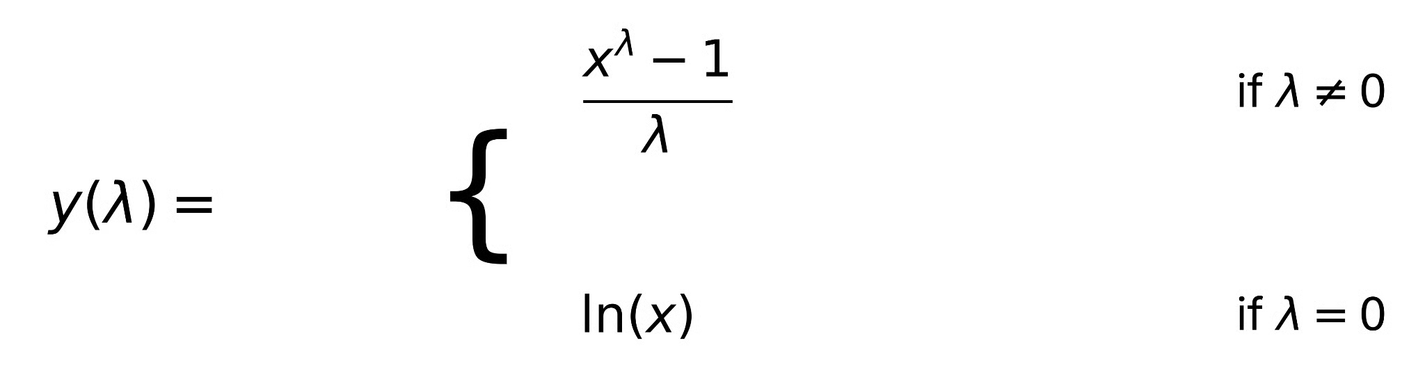
Here, x is the positive value being transformed and lambda is the transformation parameter. The (x^λ - 1) / λ form might look unfamiliar at first. That's the scaling convention that keeps the transformation continuous as lambda approaches zero. Without it, you'd have a jump discontinuity at lambda = 0 and the log case would be completely disconnected from the rest of the family. With it, the formula smoothly transitions into ln(x) as lambda → 0.

Don't worry about the derivation for now. Operationally: pick or estimate lambda, plug in your positive values, and work with the transformed output.

How to Choose Lambda for a Box-Cox Transformation

Lambda isn't something you set by hand based on intuition. You estimate it from the data. This is what distinguishes Box-Cox from just guessing "try a log." There's a principled statistical procedure underneath.

Maximum likelihood estimation

The idea is to find the lambda that makes your data best fit the assumed model. In a regression context, that means finding the lambda where the transformed response most closely satisfies the model's assumptions, typically normality and constant variance of the residuals. You're not picking the lambda that makes the marginal distribution of the response look most normal in isolation. You're picking the one that works best within the modeling context. That distinction matters, and we'll come back to it in the mistakes section.

Box-Cox profile likelihood

One of the most useful diagnostics here is the profile likelihood plot: lambda values on the x-axis, the log-likelihood on the y-axis. The peak tells you the estimated optimal lambda. Just as useful is the confidence interval around that peak, typically shown as a horizontal line at a threshold below the maximum. Any lambda inside that interval is statistically indistinguishable from the optimum.

Choosing an interpretable lambda

Here's a practical consideration that people underweight. If the optimal lambda is something like 0.43, and lambda = 0.5 falls inside the confidence interval, go with 0.5. A square-root transformation is easier to explain, easier to back-transform, and loses almost nothing in performance. The same logic applies for 0 (log) and 1 (no transformation). Interpretability matters, especially when you're explaining your model to someone who doesn't know what lambda = 0.43 means.

How to Use the Box-Cox Transformation in Python and R

Now that we know what lambda is and how it's selected, let's put this into practice. Python first, then R.

Box-Cox transformation in Python

SciPy's stats module handles this directly. The boxcox() function both estimates lambda and returns the transformed values in one call. Here's a minimal example using simulated right-skewed data:

import numpy as np
from scipy import stats

# Simulate right-skewed data (e.g., weekly sales revenue in thousands)
rng = np.random.default_rng(42)
revenue = rng.exponential(scale=50, size=300)

# Confirm all values are positive before transforming
assert (revenue > 0).all(), "Box-Cox requires strictly positive values"

# Estimate lambda and transform
transformed, estimated_lambda = stats.boxcox(revenue)

print(f"Estimated lambda: {estimated_lambda:.4f}")
print(f"Original mean: {revenue.mean():.2f}, std: {revenue.std():.2f}")
print(f"Transformed mean: {transformed.mean():.2f}, std: {transformed.std():.2f}")

The estimated_lambda here is what maximizes the log-likelihood under the normality assumption. You'd then use this same value when transforming new data for prediction.

Note that this estimates lambda from the marginal distribution of the response, not within a regression model. For a modeling workflow, you’d evaluate lambda in the model context. The R example below shows how using MASS’s boxcox() function.

Box-Cox transformation in R

In R, the MASS package's boxcox() function is built for regression workflows. It takes a fitted model object and plots the profile likelihood directly, which is a more natural fit since you're evaluating lambda in the context of a model rather than on a standalone vector.

library(MASS)

# Simulate right-skewed response (e.g., weekly revenue)
set.seed(42)
revenue <- rexp(300, rate = 1/50)
predictor <- rnorm(300)

# Fit initial model
initial_model <- lm(revenue ~ predictor)

# Estimate lambda via profile likelihood
bc_result <- boxcox(initial_model, lambda = seq(-2, 2, by = 0.1))

# Extract the lambda with highest log-likelihood
best_lambda <- bc_result$x[which.max(bc_result$y)]
cat("Best lambda:", round(best_lambda, 3), "\n")

# Refit with transformed response
revenue_transformed <- (revenue^best_lambda - 1) / best_lambda
final_model <- lm(revenue_transformed ~ predictor)

R's boxcox() plots the profile likelihood automatically, so you get the confidence interval visualization for free. That makes it easy to decide whether to round lambda to a simpler value.

How to Interpret and Reverse a Box-Cox Transformation

Once you've transformed the response and fitted a model, your predictions are on the transformed scale, not the original one. A prediction of 3.2 means 3.2 units of (x^λ - 1) / λ, not 3.2 units of revenue.

Interpreting coefficients carefully

Coefficient interpretation changes after transformation. On the transformed scale, a one-unit increase in a predictor corresponds to a certain change in y(λ), not in the original y. If lambda is close to 0 (near-log), you can approximate percentage changes in the original scale. For other values of lambda, the relationship is more involved and depends on the current level of x.

Inverse transformation

To convert predictions back to the original scale, apply the inverse:

For lambda = 0, the inverse of ln(x) is simply exp(y).

A word on retransformation bias

Back-transforming the predicted mean on the transformed scale doesn't give you an unbiased estimate of the mean on the original scale. This is a known consequence of Jensen's inequality, and it matters most in settings like forecasting mean values in log-linear models. Going deep on bias correction is beyond our scope here. Our Introduction to Regression in Python course covers prediction and interpretation in regression models more broadly if you want that context.

Box-Cox vs Other Transformations

When should you actually reach for Box-Cox versus alternatives you might already be using?

Box-Cox vs log transformation

The log transformation is the lambda = 0 case of Box-Cox. Full stop. If you've used log transformation before, you've used a specific instance of Box-Cox with lambda fixed rather than estimated. The advantage of Box-Cox is that it doesn't commit to lambda = 0 upfront. That said, if your profile likelihood peaks squarely at lambda = 0, just use a log. No reason to add complexity.

Box-Cox vs Yeo-Johnson transformation

The Yeo-Johnson transformation is a direct extension of Box-Cox designed to handle zeros and negative values. It's the one to reach for when your data includes zeros (counts, for instance) or negative values. The transformations are mathematically similar. Yeo-Johnson just relaxes the positivity constraint. In scikit-learn, PowerTransformer supports both, method='box-cox' and method='yeo-johnson', which makes switching easy to try.

Box-Cox vs standardization

Standardization (z-scoring) shifts and scales data: it changes the mean to 0 and the standard deviation to 1. Box-Cox changes the shape of the distribution through a nonlinear transformation. They solve different problems. Standardization doesn't reduce skewness or stabilize variance. Box-Cox doesn't center your data or make features comparable in magnitude. You might do both in sequence, transforming first and then standardizing, but they're not alternatives.

Limitations and Common Mistakes

Some of these are obvious in hindsight. That doesn’t stop them from happening, and a few of them are subtle enough that “obvious” is doing a lot of work.

Applying Box-Cox to zero or negative values

The formula breaks down at or below zero. 0^λ is 0 for positive lambda and undefined for negative lambda; log(0) is negative infinity. If your data has zeros or negatives, Box-Cox will either error out or silently produce nonsense. Use Yeo-Johnson instead, or add a small constant shift. The latter is an approximation worth treating with some skepticism.

Transforming data only to force normality

Box-Cox should be applied in response to a specific modeling problem: non-constant variance, poor linearity, violated residual assumptions. Using it as an automatic preprocessing step to make your marginal distribution "look normal" before fitting any model is backwards. The lambda that normalizes your response in isolation may not be the lambda that actually improves your model's residuals.

Ignoring model diagnostics

Estimating lambda is only half the job. After transforming and refitting, check your residual plots again. Box-Cox doesn't guarantee the assumptions are met. It gives you a fighting chance. If the residuals still fan out, or there's curvature, something else is going on.

Forgetting that interpretation changes

After transformation, coefficients no longer describe relationships on the original scale. This trips people up most often when reporting results or making predictions. Keep track of which scale you're working on at every step.

Evaluating lambda outside the modeling context

Lambda estimated from a univariate distribution (just looking at the histogram of your response variable) may differ from lambda estimated within a regression model. The regression-based approach is the right one. The goal is to satisfy residual assumptions, not marginal distributional assumptions.

Forgetting to apply the transformation when making predictions

When you deploy a model trained on transformed data, you have to transform new inputs the same way using the same lambda and then back-transform predictions. Skipping either step gives you predictions on the wrong scale. This sounds obvious and is still regularly forgotten.

Conclusion

Box-Cox is a family of transformations, not a single one. Lambda determines which member of that family you get, and the log transformation is just the lambda = 0 special case. Most analysts use log by default without thinking about it. Box-Cox makes that choice explicit and gives you a principled way to ask whether a different value of lambda would actually serve the model better.

Use it when you're diagnosing something specific: heteroscedasticity in the residuals, non-linearity, assumptions that clearly aren't being met. Applying it automatically to every response variable is a habit worth breaking. And if your data has zeros or negatives, that's not Box-Cox territory. That's Yeo-Johnson.

For a deeper foundation in the regression methods that Box-Cox typically supports, our Intermediate Regression in R course and our Introduction to Regression with statsmodels in Python are good next steps.