

Install pandas
Install pandas with the pip install command in your terminal. pandas 3 requires Python 3.11 or newer; on an older Python, pip installs the newest pandas 2.x release your Python supports.
Alternatively, you can install it via conda:
After installing pandas, it's good practice to check the installed version to ensure everything is working correctly:
This confirms that pandas is installed correctly and lets you verify compatibility with other packages.
What Changed in pandas 3.0 and 3.1
pandas 3.0, released in January 2026, changed how copies, strings, and assignment work, and pandas 3.1 (October 2026) deprecated most uses of inplace=True. Code from older tutorials mostly still runs, but four changes catch people out:
- Copy-on-Write is the default. Any subset or method result behaves as a copy, so changing it never changes the original DataFrame. The
SettingWithCopyWarningis gone, and so is the need for defensive.copy()calls. - Chained assignment no longer works.
df["Age"][0] = 35updates a temporary copy and leavesdfunchanged, and pandas warns with aChainedAssignmentError. Use a single.loc[]call instead. - Strings have their own data type. Text columns are now inferred as
strinstead ofobject, backed by PyArrow when it is installed. inplace=Trueis deprecated forsort_values(),reset_index(),dropna(),drop_duplicates(),rename(), and several other methods. Reassign the result instead:df = df.dropna().
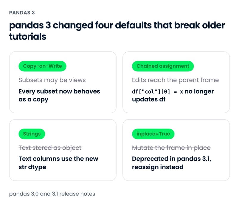
Here is the chained assignment change on a small DataFrame:
import pandas as pd
patients = pd.DataFrame({"name": ["Ana", "Ben", "Chloe"], "age": [34, 51, 28]})
patients["age"][0] = 35 # chained assignment: patients is not changed
patients.loc[0, "age"] = 35 # a single .loc[] call: patients is updated
print(patients.dtypes)name str
age int64
dtype: objectEvery example in this tutorial follows the pandas 3 rules. For the full list of changes, see the official release notes for pandas 3.0 and pandas 3.1. If you maintain older code, our guide to the SettingWithCopyWarning explains the behavior Copy-on-Write replaced.
Importing Data in pandas
To begin working with pandas, import the pandas Python package as shown below. When importing pandas, the most common alias for pandas is pd.
Importing CSV files
Use read_csv() with the path to the CSV file to read a comma-separated values file (see our tutorial on importing data with read_csv() for more detail).
This read operation loads the CSV file diabetes.csv into a pandas DataFrame named df. Throughout this tutorial, we use the Pima Indians Diabetes dataset: 768 patients, eight health measurements such as Glucose, BMI, and Age, and an Outcome column where 1 means the patient was diagnosed with diabetes.
Importing text files
Reading text files is similar to CSV files. The only nuance is that you need to specify a separator with the sep argument, as shown below. The separator is the character that separates the values (columns) on each line. Comma (sep=","), tab (sep="\t"), colon (sep=":"), and whitespace (sep=r"\s+") are the most common. r"\s+" is a regular expression that matches one or more whitespace characters; the r prefix makes it a raw string, so Python doesn't treat \s as an invalid escape sequence.
df = pd.read_csv("diabetes.txt", sep=r"\s+")Importing Excel files (single sheet)
Read Excel files with the read_excel() function, using the file path as an input. pandas needs an extra engine package for Excel: install openpyxl for .xlsx files, or xlrd for legacy .xls files.
You can also specify other arguments, such as header to specify which row becomes the DataFrame's header. It has a default value of 0, which denotes the first row as headers or column names. You can also specify column names as a list in the names argument. The index_col (default is None) argument can be used if the file contains a row index.
Note: In a pandas DataFrame or Series, the index is an identifier that points to the location of a row or column in a pandas DataFrame. In a nutshell, the index labels the row or column of a DataFrame and lets you access a specific row or column by using its index (you will see this later on). A DataFrame’s row index can be a range (e.g., 0 to 303), a time series (dates or timestamps), a unique identifier (e.g., employee_ID in an employees table), or other types of data. For columns, it's usually a string (denoting the column name).
Importing Excel files (multiple sheets)
Reading Excel files with multiple sheets is not that different. You just need to specify one additional argument, sheet_name, where you can either pass a string for the sheet name or an integer for the sheet position (note that Python uses 0-indexing, where the first sheet can be accessed with sheet_name = 0)
# Extracting the second sheet since Python uses 0-indexing
df = pd.read_excel('diabetes_multi.xlsx', sheet_name=1)Importing JSON file
Similar to the read_csv() function, you can use read_json() for JSON file types with the JSON file name as the argument (for more detail read this tutorial on importing JSON and HTML data into pandas). The below code reads a JSON file from disk and creates a DataFrame object df.
If you want to learn more about importing data with pandas, check out this cheat sheet on importing various file types with Python.
Importing data from SQL databases
To load data from a relational database, use pd.read_sql() along with a database connection.
import sqlite3

# Establish a connection to an SQLite database
conn = sqlite3.connect("my_database.db")

# Read data from a table
df = pd.read_sql("SELECT * FROM my_table", conn)For other databases, such as PostgreSQL or MySQL, pass a SQLAlchemy engine as the connection instead of a sqlite3 connection. For large tables, set the chunksize argument to read the result in batches.
Importing data from an API (JSON format)
If your data is coming from a web API, pandas can read it directly using pd.read_json():
If the API response is nested JSON, flatten it with pd.json_normalize(), which turns nested keys into dot-separated columns:
records = [
{"id": 1, "vitals": {"glucose": 148, "bmi": 33.6}},
{"id": 2, "vitals": {"glucose": 85, "bmi": 26.6}},
]
pd.json_normalize(records) id vitals.glucose vitals.bmi
0 1 148 33.6
1 2 85 26.6Exporting Data in pandas
Just as pandas can import data from various file types, it also allows you to export data into various formats. This happens especially when data is transformed using pandas and needs to be saved locally on your machine. Below is how to output pandas DataFrames into various formats.
Outputting a DataFrame into a CSV file
A pandas DataFrame (here we are using df) is saved as a CSV file using the .to_csv() method. Pass the file path, and set index=False unless you need the row index in the file (the default, index=True, writes it as an extra unnamed column). Our tutorial on saving a DataFrame to CSV covers the other arguments.
Outputting a DataFrame into a JSON file
Export DataFrame object into a JSON file by calling the .to_json() method.
Note: A JSON file stores a tabular object like a DataFrame as a key-value pair. Thus you would observe repeating column headers in a JSON file.
Outputting a DataFrame into a text file
As with writing DataFrames to CSV files, you can call .to_csv(). The only differences are that the output file format is in .txt, and you need to specify a separator using the sep argument.
Outputting a DataFrame into an Excel file
Call .to_excel() on the DataFrame to save it as an .xlsx file (this needs openpyxl). pandas can no longer write legacy .xls files.
Viewing and Understanding DataFrames in pandas
After reading tabular data as a DataFrame, you would need to have a glimpse of the data. You can either view a small sample of the dataset or a summary of the data in the form of summary statistics.
How to view data using .head() and .tail()
You can view the first few or last few rows of a DataFrame using the .head() or .tail() methods, respectively. You can specify the number of rows through the n argument (the default value is 5).
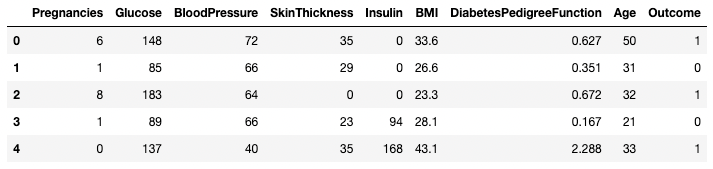
First five rows of the DataFrame
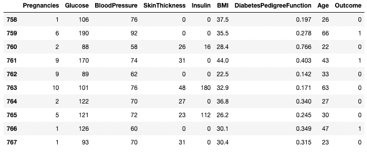
Last 10 rows of the DataFrame
Understanding data using .describe()
The .describe() method prints the summary statistics of all numeric columns, such as count, mean, standard deviation, range, and quartiles of numeric columns.
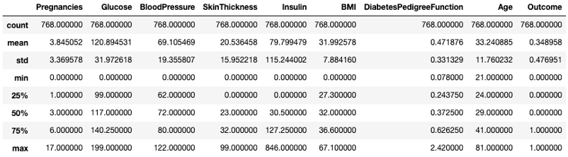
Get summary statistics with .describe()
It gives a quick look at the scale, skew, and range of numeric data.
You can also modify the quartiles using the percentiles argument. Here, for example, we’re looking at the 30%, 50%, and 70% percentiles of the numeric columns in DataFrame df.
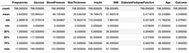
Get summary statistics with specific percentiles
You can also isolate specific data types in your summary output by using the include argument. Here, for example, we’re only summarizing the columns with the integer data type.
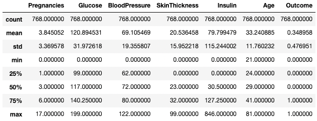
Get summary statistics of integer columns only
Similarly, you might want to exclude certain data types using exclude argument.
BMI DiabetesPedigreeFunction
count 768.000000 768.000000
mean 31.992578 0.471876
std 7.884160 0.331329
min 0.000000 0.078000
25% 27.300000 0.243750
50% 32.000000 0.372500
75% 36.600000 0.626250
max 67.100000 2.420000
Often, practitioners find it easy to view such statistics by transposing them with the .T attribute.
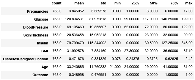
Transpose summary statistics with .T
For more on describing DataFrames, check out the following cheat sheet.
Understanding data using .info()
The .info() method is a quick way to look at the data types, missing values, and data size of a DataFrame. Here, we’re setting the show_counts argument to True, which shows the number of non-missing values in each column. We’re also setting memory_usage to True, which shows the total memory usage of the DataFrame elements. When verbose is set to True, it prints the full summary from .info().
df.info(show_counts=True, memory_usage=True, verbose=True)<class 'pandas.DataFrame'>
RangeIndex: 768 entries, 0 to 767
Data columns (total 9 columns):
# Column Non-Null Count Dtype
--- ------ -------------- -----
0 Pregnancies 768 non-null int64
1 Glucose 768 non-null int64
2 BloodPressure 768 non-null int64
3 SkinThickness 768 non-null int64
4 Insulin 768 non-null int64
5 BMI 768 non-null float64
6 DiabetesPedigreeFunction 768 non-null float64
7 Age 768 non-null int64
8 Outcome 768 non-null int64
dtypes: float64(2), int64(7)
memory usage: 54.1 KBUnderstanding your data using .shape
The number of rows and columns of a DataFrame can be identified using the .shape attribute of the DataFrame. It returns a tuple (row, column) and can be indexed to get only rows, and only columns count as output.
df.shape # Get the number of rows and columns
df.shape[0] # Get the number of rows only
df.shape[1] # Get the number of columns only(768,9)
768
9Get all columns and column names
Calling the .columns attribute of a DataFrame object returns the column names in the form of an Index object. As a reminder, a pandas index is the address/label of the row or column.
df.columnsIndex(['Pregnancies', 'Glucose', 'BloodPressure', 'SkinThickness', 'Insulin', 'BMI',
'DiabetesPedigreeFunction', 'Age', 'Outcome'],
dtype='str')It can be converted to a list using a list() function.
list(df.columns)['Pregnancies',
'Glucose',
'BloodPressure',
'SkinThickness',
'Insulin',
'BMI',
'DiabetesPedigreeFunction',
'Age',
'Outcome']Checking for missing values in pandas with .isnull()
The sample DataFrame does not have any missing values. Let's introduce a few to make things interesting. The .copy() method makes a copy of the original DataFrame. Working on a copy keeps the original df intact for the examples that follow. Using .loc (covered later), you can set the rows labeled 2 to 5 of the Pregnancies column to missing values. Because missing values are stored as NaN, a float, pandas converts the column from int64 to float64.
df2 = df.copy()
df2.loc[2:5,'Pregnancies'] = None
df2.head(7)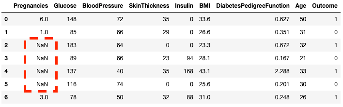
You can see, that now rows 2 to 5 are NaN
You can check whether each element in a DataFrame is missing using the .isnull() method.
df2.isnull().head(7)Given it's often more useful to know how much missing data you have, you can combine .isnull() with .sum() to count the number of nulls in each column.
df2.isnull().sum()Pregnancies 4
Glucose 0
BloodPressure 0
SkinThickness 0
Insulin 0
BMI 0
DiabetesPedigreeFunction 0
Age 0
Outcome 0
dtype: int64You can also do a double sum to get the total number of nulls in the DataFrame.
df2.isnull().sum().sum()4Sorting, Slicing, and Extracting Data in pandas
The pandas package offers several ways to sort, subset, filter, and isolate data in your DataFrames. Here, we'll see the most common ways.
Sorting data
To sort a DataFrame by a specific column, use .sort_values(). It returns a new, sorted DataFrame and leaves df unchanged, so assign the result to a variable if you want to keep it:
df.sort_values(by="Age", ascending=False) # Sort by Age in descending orderYou can sort by multiple columns:
df.sort_values(by=["Age", "Glucose"], ascending=[False, True])Resetting the index
Sorting or filtering keeps the original row labels, so the index ends up out of order. Use .reset_index() to get a fresh 0-based index (see our pandas reset index tutorial for more options):
df_sorted = df.sort_values(by="Age", ascending=False).reset_index(drop=True) # drop=True discards the old index
df_sorted[["Age", "Glucose", "Outcome"]].head(3) Age Glucose Outcome
0 81 134 0
1 72 119 0
2 70 145 1Isolating one column using [ ]
You can isolate a single column using a square bracket [ ] with a column name in it. The output is a pandas Series object. A pandas Series is a one-dimensional array containing data of any type, including integer, float, string, boolean, python objects, etc. A DataFrame is comprised of many series that act as columns.
df['Outcome']0 1
1 0
2 1
3 0
4 1
..
763 0
764 0
765 0
766 1
767 0
Name: Outcome, Length: 768, dtype: int64Isolating two or more columns using [[ ]]
You can also provide a list of column names inside the square brackets to fetch more than one column. Here, square brackets are used in two different ways. We use the outer square brackets to indicate a subset of a DataFrame, and the inner square brackets to create a list.
df[['Pregnancies', 'Outcome']] Pregnancies Outcome
0 6 1
1 1 0
2 8 1
3 1 0
4 0 1
.. ... ...
763 10 0
764 2 0
765 5 0
766 1 1
767 1 0
[768 rows x 2 columns]Isolating one row using [ ]
A single row can be fetched by passing in a boolean series with one True value. In the example below, the second row with index = 1 is returned. Here, .index returns the row labels of the DataFrame, and the comparison turns that into a Boolean one-dimensional array.
df[df.index==1]
Isolating one row in pandas
Isolating two or more rows using [ ]
Similarly, two or more rows can be returned using the .isin() method instead of a == operator.
df[df.index.isin(range(2,10))]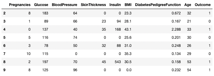
Isolating specific rows in pandas
Using .loc[] and .iloc[] to fetch rows
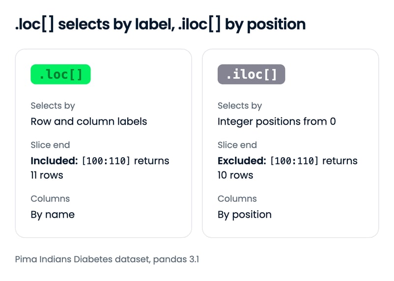
You can fetch specific rows by labels or conditions using .loc[] and .iloc[] ("location" and "integer location"). .loc[] uses a label to point to a row, column or cell, whereas .iloc[] uses the numeric position. Our loc vs iloc guide covers every difference; to see the main one here, let’s change the index of df2 created earlier so labels and positions no longer match.
df2.index = range(1,769)The below example returns a pandas Series instead of a DataFrame. In .loc[1], 1 is a label, so it returns the row labeled 1 (the first row after re-indexing). In .iloc[1], 1 is a zero-based position, so it returns the second row, which carries the label 2.
df2.loc[1]Pregnancies 6.000
Glucose 148.000
BloodPressure 72.000
SkinThickness 35.000
Insulin 0.000
BMI 33.600
DiabetesPedigreeFunction 0.627
Age 50.000
Outcome 1.000
Name: 1, dtype: float64df2.iloc[1]Pregnancies 1.000
Glucose 85.000
BloodPressure 66.000
SkinThickness 29.000
Insulin 0.000
BMI 26.600
DiabetesPedigreeFunction 0.351
Age 31.000
Outcome 0.000
Name: 2, dtype: float64You can also fetch multiple rows by providing a range in square brackets. The two accessors treat the end of the range differently: .loc[100:110] includes label 110 and returns 11 rows, while .iloc[100:110] stops before position 110 and returns 10 rows.
df2.loc[100:110]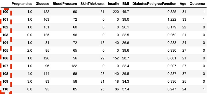
Isolating rows in pandas with .loc[]
df2.iloc[100:110]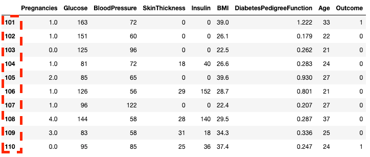
Isolating rows in pandas with .iloc[]
You can also subset with .loc[] and .iloc[] by using a list instead of a range.
df2.loc[[100, 200, 300]]
Isolating rows using a list in pandas with .loc[]
df2.iloc[[100, 200, 300]]
Isolating rows using a list in pandas with .iloc[]
You can also select specific columns along with rows. This is where .iloc[] is different from .loc[] – it requires column location and not column labels.
df2.loc[100:110, ['Pregnancies', 'Glucose', 'BloodPressure']] Pregnancies Glucose BloodPressure
100 1.0 122 90
101 1.0 163 72
102 1.0 151 60
103 0.0 125 96
104 1.0 81 72
105 2.0 85 65
106 1.0 126 56
107 1.0 96 122
108 4.0 144 58
109 3.0 83 58
110 0.0 95 85df2.iloc[100:110, :3] Pregnancies Glucose BloodPressure
101 1.0 163 72
102 1.0 151 60
103 0.0 125 96
104 1.0 81 72
105 2.0 85 65
106 1.0 126 56
107 1.0 96 122
108 4.0 144 58
109 3.0 83 58
110 0.0 95 85For faster workflows, you can pass in the starting index of a row as a range.
df2.loc[760:, ['Pregnancies', 'Glucose', 'BloodPressure']] Pregnancies Glucose BloodPressure
760 6.0 190 92
761 2.0 88 58
762 9.0 170 74
763 9.0 89 62
764 10.0 101 76
765 2.0 122 70
766 5.0 121 72
767 1.0 126 60
768 1.0 93 70df2.iloc[760:, :3] Pregnancies Glucose BloodPressure
761 2.0 88 58
762 9.0 170 74
763 9.0 89 62
764 10.0 101 76
765 2.0 122 70
766 5.0 121 72
767 1.0 126 60
768 1.0 93 70You can update values by combining .loc[] with the assignment operator =. Build the condition from the same DataFrame you are updating: a condition built from df no longer lines up with the new index of df2, and pandas raises an error.
df2.loc[df2["Age"] == 81, "Age"] = 80Filtering rows with conditions
pandas lets you filter data by conditions over row/column values. For example, the below code selects the row where Blood Pressure is exactly 122. Here, we are isolating rows using the brackets [ ] as seen in previous sections. However, instead of inputting row indices or column names, we are inputting a condition where the column BloodPressure is equal to 122. We denote this condition using df.BloodPressure == 122.
df[df.BloodPressure == 122]
Isolating rows based on a condition in pandas
The below example fetches all rows where Outcome is 1. Here df.Outcome selects that column, df.Outcome == 1 returns a Series of Boolean values determining which Outcomes are equal to 1, then [] takes a subset of df where that Boolean Series is True.
df[df.Outcome == 1]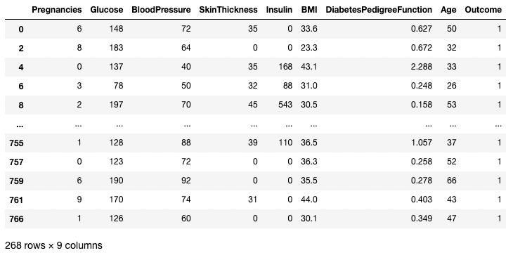
Isolating rows based on a condition in pandas
You can use a > operator to draw comparisons. The below code fetches Pregnancies, Glucose, and BloodPressure for all records with BloodPressure greater than 100.
df.loc[df['BloodPressure'] > 100, ['Pregnancies', 'Glucose', 'BloodPressure']] Pregnancies Glucose BloodPressure
43 9 171 110
84 5 137 108
106 1 96 122
177 0 129 110
207 5 162 104
362 5 103 108
369 1 133 102
440 0 189 104
549 4 189 110
658 11 127 106
662 8 167 106
672 10 68 106
691 13 158 114Cleaning Data in pandas
Data cleaning is one of the most common tasks in data science. pandas lets you preprocess data for any use, including but not limited to training machine learning and deep learning models. Let’s use the DataFrame df2 from earlier, having four missing values, to illustrate a few data cleaning use cases. As a reminder, here's how you can see how many missing values are in a DataFrame.
df2.isnull().sum()Pregnancies 4
Glucose 0
BloodPressure 0
SkinThickness 0
Insulin 0
BMI 0
DiabetesPedigreeFunction 0
Age 0
Outcome 0
dtype: int64Dealing with missing data technique #1: Dropping missing values
One way to deal with missing data is to drop it. This is particularly useful in cases where you have plenty of data and losing a small portion won’t impact the downstream analysis. You can use a .dropna() method as shown below. Here, we are saving the results from .dropna() into a DataFrame df3.
df3 = df2.copy()
df3 = df3.dropna()
df3.shape(764, 9) # this is 4 rows less than df2The axis argument lets you specify whether you are dropping rows, or columns, with missing values. The default axis removes the rows containing NaNs. Use axis = 1 to remove the columns with one or more NaN values. As in every example in this tutorial, we reassign the result instead of passing inplace=True, which pandas 3.1 deprecates for .dropna().
df3 = df2.dropna(axis=1)
list(df3.columns)['Glucose', 'BloodPressure', 'SkinThickness', 'Insulin', 'BMI', 'DiabetesPedigreeFunction', 'Age', 'Outcome']By default, .dropna() drops a row if any of its values is missing. Set the how argument to 'all' to drop only rows where every value is missing. No row in df2 is completely empty, so nothing is dropped:
df3 = df2.dropna(how="all")
df3.shape(768, 9)Dealing with missing data technique #2: Replacing missing values
Instead of dropping missing values, you can replace them with a summary statistic or a fixed value. For example, if one day is missing from a week of temperature readings, filling it with that week's average keeps the row and loses little information. The code below fills the missing Pregnancies values with that column's mean.
df3 = df2.copy()
# Get the mean of Pregnancies
mean_value = df3["Pregnancies"].mean()
# Fill only that column's missing values
df3["Pregnancies"] = df3["Pregnancies"].fillna(mean_value)
df3["Pregnancies"].head(7)1 6.000000
2 1.000000
3 3.846859
4 3.846859
5 3.846859
6 3.846859
7 3.000000
Name: Pregnancies, dtype: float64Dealing with duplicate data
Let's add some duplicates to the original data to learn how to eliminate duplicates in a DataFrame. Here, we use the pd.concat() function to concatenate the rows of the df2 DataFrame to the df2 DataFrame, adding perfect duplicates of every row in df2.
df3 = pd.concat([df2, df2])
df3.shape(1536, 9)You can remove all duplicate rows (default) from the DataFrame using .drop_duplicates() method.
df3 = df3.drop_duplicates()
df3.shape(768, 9)Renaming columns
A common data cleaning task is renaming columns. Pass the .rename() method a columns dictionary that maps old names to new ones:
df3 = df3.rename(columns={"DiabetesPedigreeFunction": "DPF"})
df3[["Glucose", "BMI", "DPF", "Age"]].head() Glucose BMI DPF Age
1 148 33.6 0.627 50
2 85 26.6 0.351 31
3 183 23.3 0.672 32
4 89 28.1 0.167 21
5 137 43.1 2.288 33You can also assign a full list of names to .columns. The list must name every column in its current order: pandas assigns names by position, so a list in the wrong order silently mislabels your data.
df3.columns = ["Pregnancies", "Glucose", "BloodPressure", "SkinThickness", "Insulin", "BMI", "DPF", "Age", "Outcome"]
list(df3.columns)['Pregnancies', 'Glucose', 'BloodPressure', 'SkinThickness', 'Insulin', 'BMI', 'DPF', 'Age', 'Outcome']For more on data cleaning, and for easier, more predictable data cleaning workflows, check out the following checklist, which provides you with a comprehensive set of common data cleaning tasks.
Combining DataFrames in pandas
pandas combines DataFrames in two ways: .merge() joins tables on shared key columns, like a SQL join, and pd.concat() stacks tables on top of or next to each other.
Merging DataFrames with .merge()
Use .merge() when two tables share a key column. Suppose a second table maps each Outcome code to a readable label. A left merge on Outcome adds that label to every patient row:
outcome_labels = pd.DataFrame({"Outcome": [0, 1], "Diagnosis": ["Non-diabetic", "Diabetic"]})
df_labeled = df.merge(outcome_labels, on="Outcome", how="left")
df_labeled[["Glucose", "Outcome", "Diagnosis"]].head(3) Glucose Outcome Diagnosis
0 148 1 Diabetic
1 85 0 Non-diabetic
2 183 1 DiabeticThe how argument sets the join type: "left" keeps every row of df, "inner" keeps only rows with a match in both tables, and "outer" keeps all rows from both. Our tutorial on joining DataFrames in pandas covers .join() and every join type in detail.
Concatenating DataFrames with pd.concat()
Use pd.concat() when tables have the same columns and you want to stack their rows, for example patient records that arrive in two batches. Set ignore_index=True to get a fresh 0-based index instead of keeping each batch's labels:
batch_1 = df.iloc[:500]
batch_2 = df.iloc[500:]
df_combined = pd.concat([batch_1, batch_2], ignore_index=True)
df_combined.shape(768, 9)With axis=1, pd.concat() places tables side by side instead, matching rows by their index labels:
measurements = df[["Glucose", "BMI"]]
outcomes = df[["Outcome"]]
pd.concat([measurements, outcomes], axis=1).head(3) Glucose BMI Outcome
0 148 33.6 1
1 85 26.6 0
2 183 23.3 1For hands-on practice with both methods, try our Joining Data with pandas course.
Data Analysis in pandas
The main value proposition of pandas lies in its quick data analysis functionality. In this section, we'll focus on a set of analysis techniques you can use in pandas.
Summary operators (mean, mode, median)
As you saw earlier, you can get the mean of each column value using the .mean() method.
df.mean()Pregnancies 3.845052
Glucose 120.894531
BloodPressure 69.105469
SkinThickness 20.536458
Insulin 79.799479
BMI 31.992578
DiabetesPedigreeFunction 0.471876
Age 33.240885
Outcome 0.348958
dtype: float64A mode can be computed similarly using the .mode() method.
df.mode()
Printing the mode of columns in pandas
Similarly, the median of each column is computed with the .median() method
df.median()Pregnancies 3.0000
Glucose 117.0000
BloodPressure 72.0000
SkinThickness 23.0000
Insulin 30.5000
BMI 32.0000
DiabetesPedigreeFunction 0.3725
Age 29.0000
Outcome 0.0000
dtype: float64Create new columns based on existing columns
pandas provides fast and efficient computation by combining two or more columns like scalar variables. The below code divides each value in the column Glucose with the corresponding value in the Insulin column to compute a new column named Glucose_Insulin_Ratio.
df2['Glucose_Insulin_Ratio'] = df2['Glucose']/df2['Insulin']
df2.head()
Create a new column from existing columns in pandas
Rows where Insulin is 0 show inf, because dividing by zero gives infinity. In this dataset, a 0 for Insulin means the measurement is missing (374 of the 768 rows), so treat those zeros as missing before dividing:
df2["Glucose_Insulin_Ratio"] = df2["Glucose"] / df2["Insulin"].where(df2["Insulin"] > 0)
df2["Glucose_Insulin_Ratio"].head()1 NaN
2 NaN
3 NaN
4 0.946809
5 0.815476
Name: Glucose_Insulin_Ratio, dtype: float64.where() keeps values that meet the condition and replaces the rest with NaN, so the ratio is missing instead of infinite for those rows. Our tutorial on adding columns in pandas shows more ways to derive new columns.
Counting using .value_counts()
When a column holds categories, you often want to count how many observations fall into each one. The .value_counts() method does this. Here, for example, we are counting the number of observations where Outcome is diabetic (1) and the number of observations where the Outcome is non-diabetic (0).
df['Outcome'].value_counts()Outcome
0 500
1 268
Name: count, dtype: int64Adding the normalize argument returns proportions instead of absolute counts.
df['Outcome'].value_counts(normalize=True)Outcome
0 0.651042
1 0.348958
Name: proportion, dtype: float64
Turn off automatic sorting of results using sort argument (True by default). The default sorting is based on the counts in descending order.
df['Outcome'].value_counts(sort=False)Outcome
1 268
0 500
Name: count, dtype: int64You can also apply .value_counts() to a DataFrame object and specific columns within it instead of just a column. Here, for example, we are applying value_counts() on df with the subset argument, which takes in a list of columns.
df.value_counts(subset=['Pregnancies', 'Outcome'])Pregnancies Outcome
1 0 106
2 0 84
0 0 73
3 0 48
4 0 45
0 1 38
5 0 36
6 0 34
1 1 29
3 1 27
7 1 25
4 1 23
8 1 22
5 1 21
7 0 20
2 1 19
9 1 18
6 1 16
8 0 16
10 0 14
1 10
9 0 10
11 1 7
13 0 5
1 5
12 0 5
11 0 4
12 1 4
14 1 2
15 1 1
17 1 1
Name: count, dtype: int64Aggregating data with .groupby() in pandas
pandas lets you aggregate values by grouping them by specific column values. You can do that by combining the .groupby() method with a summary method of your choice. The below code displays the mean of each of the numeric columns grouped by Outcome.
df.groupby('Outcome').mean()
Aggregating data by one column in pandas
.groupby() enables grouping by more than one column by passing a list of column names, as shown below.
df.groupby(['Pregnancies', 'Outcome']).mean()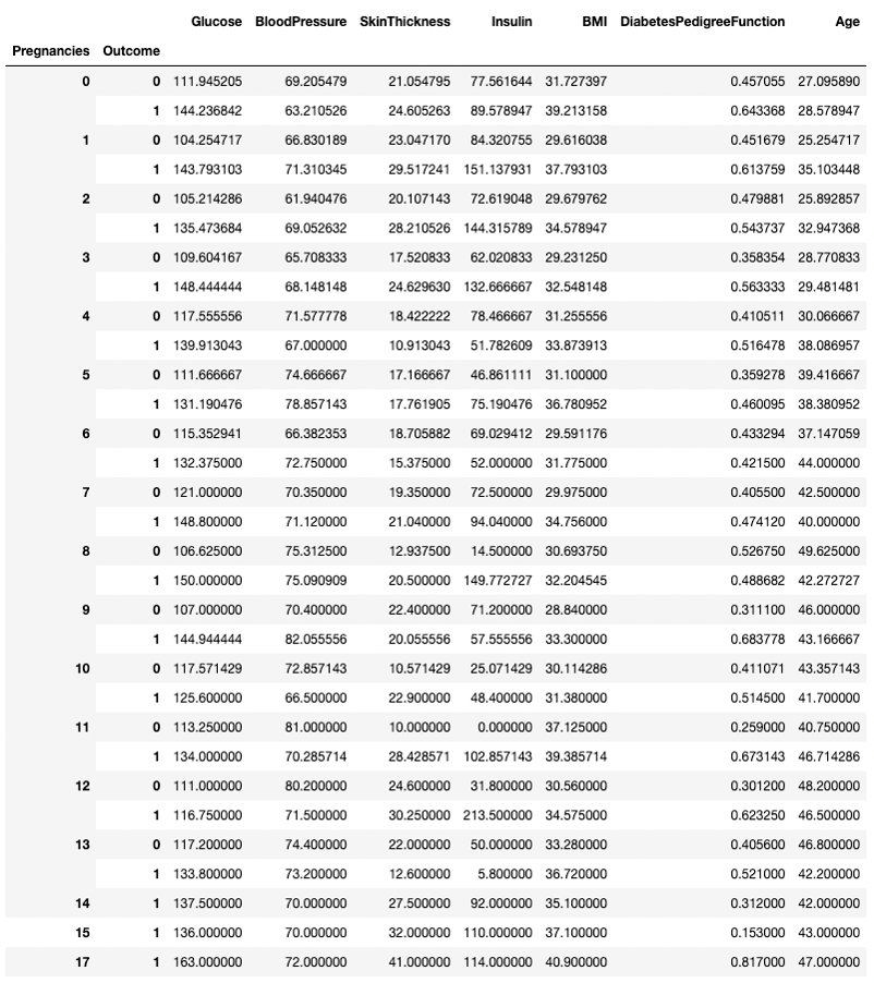
Aggregating data by two columns in pandas
Any summary method can be used alongside .groupby(), including .min(), .max(), .mean(), .median(), .sum(), and more. Our pandas GroupBy tutorial covers multiple aggregations with .agg() and other patterns.
Pivot tables
pandas also enables you to calculate summary statistics as pivot tables. This makes it easy to draw conclusions based on a combination of variables. The below code picks the rows as unique values of Pregnancies, the column values are the unique values of Outcome, and the cells contain the average value of BMI in the corresponding group.
For example, for Pregnancies = 5 and Outcome = 0, the average BMI turns out to be 31.1.
pd.pivot_table(df, values="BMI", index='Pregnancies',
columns=['Outcome'], aggfunc='mean')Outcome 0 1
Pregnancies
0 31.727397 39.213158
1 29.616038 37.793103
2 29.679762 34.578947
3 29.231250 32.548148
4 31.255556 33.873913
5 31.100000 36.780952
6 29.591176 31.775000
7 29.975000 34.756000
8 30.693750 32.204545
9 28.840000 33.300000
10 30.114286 31.380000
11 37.125000 39.385714
12 30.560000 34.575000
13 33.280000 36.720000
14 NaN 35.100000
15 NaN 37.100000
17 NaN 40.900000Data Visualization in pandas
pandas provides convenience wrappers to Matplotlib plotting functions to make it easy to visualize your DataFrames. Below, you'll see how to do common data visualizations using pandas.
Line plots in pandas
pandas enables you to chart out the relationships among variables using line plots. Below is a line plot of BMI and Glucose versus the row index.
df[['BMI', 'Glucose']].plot.line()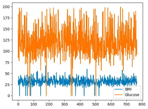
Basic line plot with pandas
You can select the choice of colors by using the color argument.
df[['BMI', 'Glucose']].plot.line(color={"BMI": "red", "Glucose": "blue"})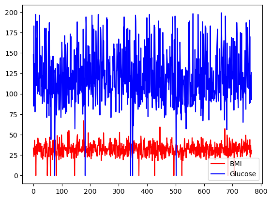
Basic line plot with pandas, with custom colors
All the columns of df can also be plotted on different scales and axes by using the subplots argument.
df.plot.line(subplots=True)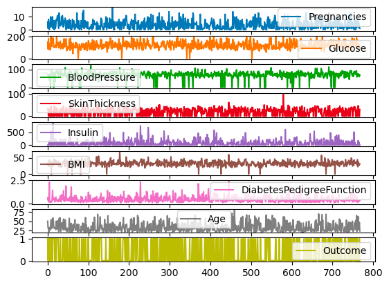
Subplots for line plots with pandas
Bar plots in pandas
For discrete columns, you can use a bar plot over the category counts to visualize their distribution. The variable Outcome with binary values is visualized below.
df['Outcome'].value_counts().plot.bar()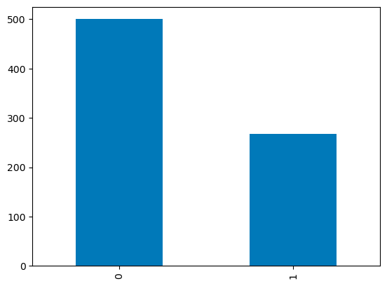
Barplots in pandas
Box plots in pandas
The quartile distribution of continuous variables can be visualized using a boxplot. The code below lets you create a boxplot with pandas.
df.boxplot(column=['BMI'], by='Outcome')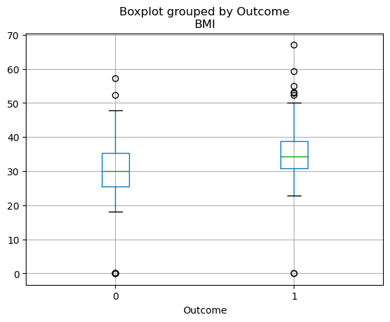
Boxplots in pandas
Final Thoughts
You now have the core pandas workflow: read a file into a DataFrame, inspect it with .head(), .info(), and .describe(), select rows with .loc[] and .iloc[], clean missing values and duplicates, merge tables, and summarize with .groupby() and pivot tables.
If you learned pandas before 2026, one habit is worth changing: reassign results instead of passing inplace=True, and make every update with a single .loc[] call. The fastest way to make the rest stick is to repeat the workflow on a dataset you care about. These resources help you go further:
- [Cheat Sheets] A plethora of Python and pandas cheat sheets to reference throughout your learning
- [Live trainings] Our free live code-along sessions, many of which use pandas
- [Courses] Data Manipulation with pandas and Joining Data with pandas for interactive practice
- [Interview prep] Our top pandas interview questions to test what you know
- [More tutorials] Check out our remaining tutorials on pandas and the PyData ecosystem, including how to implement moving averages in pandas and using the pandas .apply() method
pandas FAQs
What is pandas in Python?
pandas is an open-source Python library for working with tabular data. Its two core data structures, the DataFrame (a table) and the Series (a single column), come with functions for importing, cleaning, reshaping, aggregating, and plotting data, which is why it is the standard tool for data analysis in Python.
Why should I learn pandas?
If you're working with data in Python, pandas is pretty much a must-learn. It simplifies the process of handling and analyzing data, so you can focus on extracting insights and creating value. Whether you're dealing with small datasets or large-scale data, pandas will make your life easier with its speed, flexibility, and user-friendly data structures.
How do I install pandas?
Run pip install pandas in your terminal, or conda install pandas if you use conda. pandas 3 requires Python 3.11 or newer. Anaconda includes pandas by default, and DataCamp's DataLab has it pre-installed.
What are the basic data structures in pandas?
The two primary data structures in pandas are the Series and DataFrame. A Series is essentially a column, and a DataFrame is a two-dimensional table made up of a collection of Series. These structures are flexible, meaning they can hold data of different types (e.g., integer, string, float).
Is pandas good for large datasets?
pandas handles millions of rows comfortably, as long as the data fits in your computer's memory. For data that doesn't, read it in batches with the chunksize argument, or switch to a tool built for larger data, such as Polars, Dask, or PySpark.
How do I import data into pandas?
pandas can read data from various file formats like CSV, Excel, SQL databases, JSON, and more. The commands pd.read_csv(), pd.read_excel(), pd.read_sql(), and pd.read_json() are used for importing data from respective file types. All these commands return a DataFrame, which you can manipulate using pandas.
What changed in pandas 3.0?
pandas 3.0, released in January 2026, made Copy-on-Write the default, so every subset behaves as a copy and chained assignment such as df["col"][0] = x no longer updates the original DataFrame. It also infers text columns as a dedicated str data type instead of object, and it requires Python 3.11 or newer. pandas 3.1 then deprecated inplace=True for methods like dropna() and sort_values().
What is the difference between loc and iloc in pandas?
.loc[] selects rows and columns by label, and .iloc[] selects them by integer position, starting at 0. Slices also differ: .loc[100:110] includes the end label, while .iloc[100:110] stops before position 110. See our loc vs iloc guide for more examples.
How do I merge two DataFrames in pandas?
Use df1.merge(df2, on="key", how="left") to join two DataFrames on a shared column, the way a SQL join does. The how argument picks the join type ("left", "right", "inner", or "outer"). To stack DataFrames instead, use pd.concat().

I am an AI Strategist and Ethicist working at the intersection of data science, product, and engineering to build scalable machine learning systems. Listed as one of the "Top 200 Business and Technology Innovators" in the world, I am on a mission to democratize machine learning and break the jargon for everyone to be a part of this transformation.



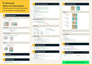




pandas is the standard Python package for data analysis, with more than 500 million downloads a month on PyPI. It reads and writes CSV, Excel, JSON, SQL, and many other formats, and its functions cover the everyday work of cleaning, reshaping, aggregating, and plotting tabular data.
In this pandas tutorial, we walk through the full workflow on one real dataset: installing pandas, importing and exporting data, inspecting a DataFrame, selecting and filtering rows, cleaning missing values and duplicates, combining tables, aggregating, and plotting. Every example runs on pandas 3.1, the current release, and we flag the pandas 3 changes that break code from older tutorials.
You need basic Python and no prior pandas experience. For a longer learning plan, see our post on how to learn pandas, and for interactive practice, our Data Manipulation with pandas course.
TL;DR
pip install pandas; pandas 3 needs Python 3.11 or newer..loc[]selects by label,.iloc[]by position..loc[]call.df = df.dropna()) instead of using the deprecatedinplace=True.What Is pandas?
pandas is a data manipulation package in Python for tabular data. That is, data in the form of rows and columns, also known as DataFrames. Intuitively, you can think of a DataFrame as an Excel sheet.
pandas’ functionality includes data transformations, like sorting rows and taking subsets, to calculating summary statistics such as the mean, reshaping DataFrames, and joining DataFrames together. pandas works well with other popular Python data science packages, often called the PyData ecosystem, including
What Is pandas Used For?
pandas is used throughout the data analysis workflow. With pandas, you can:
pandas also contains functionality for time series analysis and analyzing text data.
Key Benefits of pandas
pandas has five practical advantages for everyday data work:
How to Install pandas
Before using pandas, you need to install it. You can skip this step by registering for a free DataCamp account and using DataLab, a cloud-based IDE that comes with pandas (alongside the top Python data science packages) pre-installed.